Back to POSTS

SW engineering meets mathematical modeling - Modelica basics

by Marco Bonvini on Saturday October 22, 2016

Ask any engineer, and they’ll tell you - “It’s tough to model the real world!” Engineers perform a delicate balancing act when they create complex models of physical systems, building detailed simulations while at the same time struggling against overwhelming complexity or irrelevant detail.

Fortunately, there’s help. In this post I give an overview of the Modelica modeling language and the features that make it the right choice for modeling complex engineering systems. Modelica is not some abstract academic toy disregarded by the modern industry. In fact, in the last few years Modelica has been adopted by some of the world’s biggest automotive companies – Audi, BMW, Daimler, Ford, Toyota, and VW. These companies use Modelica to design energy efficient vehicles, improve air conditioning systems, even (in the case of the Ferrari F1 team) design racing cars! And the automotive sector is just one of many that find this language effective.

As described on the Modelica association website, Modelica is a non-proprietary, object-oriented, equation based language to conveniently model complex physical systems including a variety of different aspects, including mechanical, electrical, electronic, hydraulic, thermal, control, electric power or process-oriented subcomponents.

The concept is simple. Modelica is a language for modelling systems that can be described with equations such as

• differential equations,
• algebraic equations,
• difference equations, and
• discrete event systems

The following diagram shows the big picture behind any Modelica model

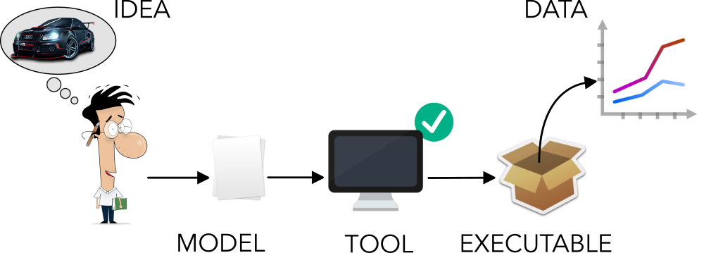
The steps are the following:

1. an engineer/scientist writes a Modelica model that represents an idea as a series of equations,
2. a Modelica tool analyzes the model and verifies its correctness – Does the model have the same number of variables and equations? Are there typos?
3. the tool compiles the model and generates an executablea
4. run the executable to simulate the system and produce data.

First example

Before diving into some of Modelica’s core concepts let’s start with an example, a kind of HelloWorld of differential equations. We’ll use the simplest differential equation you can imagine

with initial condition \( x(t_0) = 5 \)

 1 model HelloWorld  "The simplest differential equation ever"
 2   // Define variables and parameters here...
 3   Real x
 4     "The unknown variable";
 5   constant Real a = -2.0
 6     "Constant that characterizes the model";
 7   parameter Real x_start = 5.0
 8     "Initial value of the variable x";
 9 initial equation
10   // Define initial conditions here...
11   x = x_start;
12 equation
13   // Write the equations here...
14   der(x) = a*x;
15 end HelloWorld;

The keyword model defines the beginning of a model named HelloWorld. The model is divided in three sections: declarations, initializations and equations. The model starts by declaring variables, constants and parameters. Variables represent quantities that are expected to change over time. Constants, meanwhile, are fixed quantities that will never change. And finally parameters are quantities that do not change over time but may change between simulations. In this case parameter x_start, constant a and variable x have the same type, Real type meaning a real floating point number.

The keywords initial equation introduce the second part of our model. Here we define the initial conditions of the system, for example the value of x at the beginning of our model’s simulation time.

The keyword equation introduces the third and final part of our program, where we finally get down to writing the equations of the system. In this case there is one variable x and one differential equation der(x) = a*x.

One important thing to note is the der(...) operator that indicates the time derivative of the expression inside the brackets. The ability to express derivatives in such a clean and concise way is very helpful when dealing with mathematical models.

Modelica’s key principles

So we’ve completed a simple example to get familiar with Modelica. Now, let’s look at some of its most interesting features. As I mentioned at the beginning of the post, Modelica is an Object-Oriented equation-based modeling language. What exactly do those words mean? Let’s have a look, keeping in the context of mathematical modeling.

Equation-based modeling

Computer programs are nothing but clever set of instructions to let a computer solve a particular problem for us (If this sounds familiar, bear with me. I’m going to make a distinction between assignments and equations that you might not be familiar with). Let’s consider the following problem: given two numbers compute their sum. The following code snippet shows a solution to the problem implemented in C

int main(void){
  int a, b, c;
  a = 4;
  b = 3;
  c = a + b;
  return 0;
}

What happens here when the program is executed is that the value 4 is inserted in the memory space associated to variable a, the value 3 is inserted in the memory space associated to variable b and then their sum is assigned to the memory space associated to variable c.

Given the initial problem this program implements a particular solution to it. And, most of the time when we write algorithms we are writing specific solutions to certain problems. In this case the problem and its algorithmic solution were pretty straightforward!

Now here’s the kicker: when dealing with mathematical modeling the situation is quite different. You typically start with a set of equations that describe the general understanding of the system you want to model.

Then, you can collected data about that system, and feed it into those equations to start generating some interesting answers to your questions. Often there are multiple questions to answer, so the model should be as general as possible so that it can be be easily manipulated to answer all the questions.

Let’s get back to our problem: given two numbers compute their sum. The following is a Modelica model that solves it

1 model Sum
2    Integer a, b, c;
3 equation
4    c - (a + b) = 0;
5    a = 4;
6    b - 3 = 0;
7 end Sum;

The content of line 4 is the essence of equation-based modeling. It all boils down to two concepts:

• c - (a + b) = 0 is an equation and equations are not assignment like the ones we’re used to write in C, Java, Python, etc.
• a = 4 and b - 3 = 0 are located on lines 5 and 6. Both lines come after the first equation because equations are not assignment, their order does not matter. The only thing that matters is that there are the same number of variables and equations.

So it turns out that equation-based modeling is all about writing equations with code. The Modelica tool of choice will know how to symbolically analyze the model, extract equations, substitute variables in equations, sort them and apply the proper numerical methods to find the solution. The trick is knowing how the Modelica compiler works so that the model we create has better numerical properties and is therefore solved more efficiently.

Working with Causality

The equation-based paradigm opens the door to an interesting concept called a-causality.

Before focusing on the meaning and implications of a-causality let’s have a look at an example based on Newton’s second law

The acceleration of an object as produced by a net force is directly proportional to the magnitude of the net force, in the same direction as the net force, and inversely proportional to the mass of the object.

Sir Isaac Newton

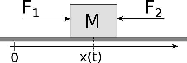
Newton’s second law describes a relationship between the following quantities: the forces acting on a body, the mass of the body and its acceleration.

The example below shows a system where a body that can move only along one direction and two forces are acting on it

Given this system, we can identify a number of problems to solve. Identifying a problem and finding its solution requires us follow a specific mental process:

• identify the known variables,
• rewrite Newton’s second law to find the desired quantity (e.g., acceleration, force, mass, etc.)

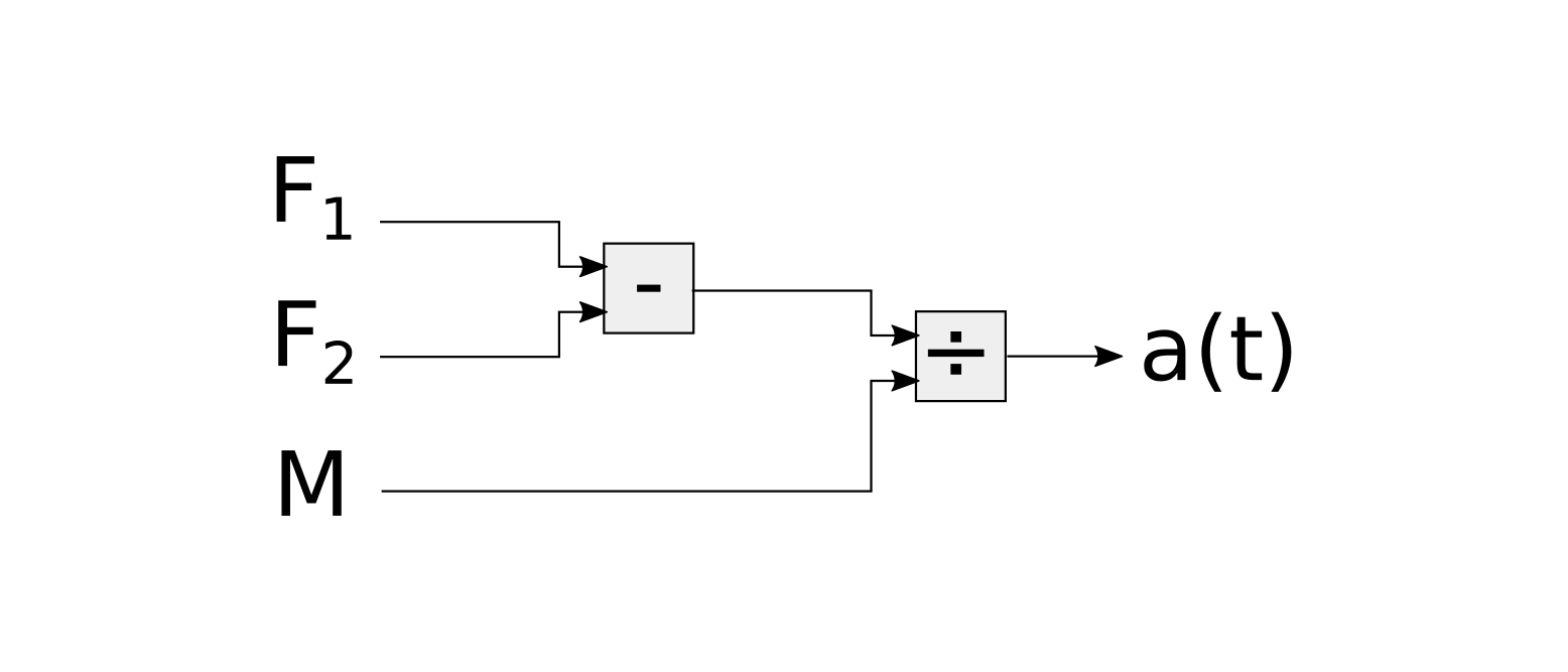
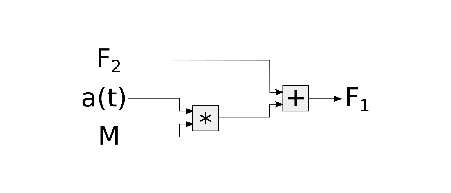
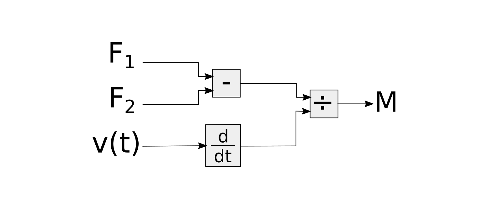
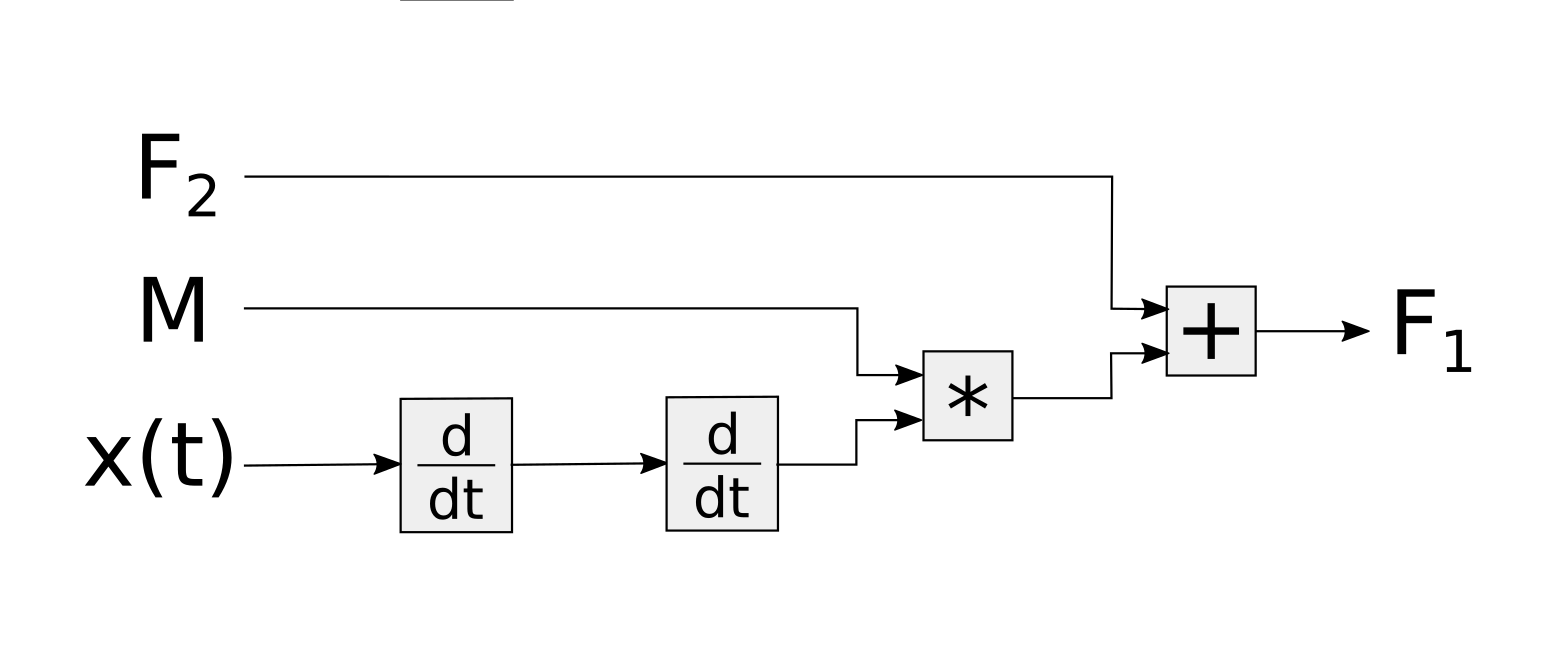
Here’s a small list of questions and their solutions presented with block diagrams; each diagram visually describes how the information flows from the inputs (i.e., known variables) to the output (i.e., answer to the question).

• given the mass, and the two forces compute the acceleration of the body

$$ a(t) =\frac{ F_1 - F_2}{M} $$

• given the mass, acceleration and one force compute the other force

$$ F_1 = F_2 + a(t) \, M$$

• given the two forces and the velocity of the body compute its mass

$$ M = \frac{F_1 - F_2}{\frac{d v(t)}{dt}} $$

• given the position of the body, the mass, and one force compute the other force

$$ F_1 = F_2 + M \, \frac{d^2 \, x(t)}{dt^2}$$

This process requires a person that looks at the problem and

1. identifies relationships between the things that are known and the results to be found,
2. rearranges Newton’s second law in order to find a path that leads from one to the other.

What we’ve just seen is the so called causal approach: explicitly describe cause-effect relationships between variables and hard-code them in an algorithm that computes the solution. Even if the physical system is always the same, a slightly different question about the system might require a complete rewrite of the algorithm that solves the problem. The block diagrams above show this concept very well. Even if the underlying system is always the same, the type of operations performed on the data and the order of those operations continuously change. This is rather inconvenient, especially when dealing with systems that are more complicated than a single body and a couple of forces!

Moreover, the design process of any complex system is an iterative process. New questions come up as the process continues. Having an algorithm that answers only one question and that needs to be completely rewritten to answer a slightly different one is practically useless.

Modelica’s equation-based nature enables the so called a-causal modelling approach: build mathematical models without imposing a priori cause-effect relationships between variables. Let’s try to model the same single body system in Modelica and see what it looks like.

 1 model SingleBodySystem
 2    Real M "The mass of the body";
 3    Real x "The position of the body";
 4    Real v "The velocity of the body";
 5    Real a "Acceleration of the body";
 6    Real F1, F2 "Forces acting on the body";
 7 initial equation
 8    // Initial conditions
 9    x = 0 "The position of the body is x=0 at time=0";
10    v = 0 "The body is not moving when time=0";
11 equation
12    // The dynamic behaviour of the system
13    der(x) = v;
14    der(v) = a;
15    M*a = F1 - F2;
16 
17    // The boundary conditions
18    F1 = 1.2;
19    F2 = 2.0;
20    M  = 5.0;
21 
22 end SingleBodySystem;

The equation section is divided in two parts. The first part describes Newton’s second law, i.e. the dynamic of the system. This part is not going to change unless the body starts moving at the speed of light!

The second part contains the boundary conditions. The boundary conditions are required to have a complete picture of the system. The boundary conditions can change from time to time depending on the question being asked.

When boundary conditions change the Modelica tool does all the hard work to finding causal relationships between the variables. Once the Modelica tools finally finds the relationships between inputs and outputs it generates an executable that solves the problem.

Such an approach leverages a computer for doing the boring and error prone job of rewriting and sorting equations. Computers are definitely better than humans at doing this!

A biproduct of A-causality is that models written in Modelica are more readable and maintainable. The model contains a description of the system and its boundary conditions rather than a solution to a specific problem. Most of the readers familiar with software engineering best practices know this is very important, especially when dealing with complex and large models.

After this brief discussion on a-causality I hope you’re convinced that writing ad-hoc solution to problems is almost as bad as writing assembly code without using a higher level language and a compiler.

Conclusion

In this post we just started scratching the surface. We learned a bit of Modelica syntax and we’ve seen that Modelica works directly with equations and that this leads to model that are a-causal. A-causal models are more readable and more flexible and are a good way to express complex engineering problems.

The next post SW engineering meets mathematical modeling - Types and Objects goes a little bit deeper and explains the meaning of Object-Oriented modeling as well some nice features related to Modelica’s type system.

If after reading this post you’re even more interested in Modelica I suggest you to look at the online book Modelica by examples by Michael Tiller, otherwise browse the website of the Modelica associations www.modelica.org.

If you’re interested in the work I’ve done with Modelica over the last years you can look here.

Aknowledgments

Special thanks to Daniel McQuillen for proof reading this post and providing helpful suggestions.

Back to POSTS