Back to POSTS

All about Modelica

by Marco Bonvini on Monday June 29, 2020

Early in my career, when ML and AI weren’t as cool, I fell in love with modeling and simulations. As Joel Spolsky recently put it, sometimes you’re working on something that’s just too complicated to reason about with simple math, you can’t even begin to guess how the inputs affect the outputs. In such cases, simulation models will help you understand better complex problems.

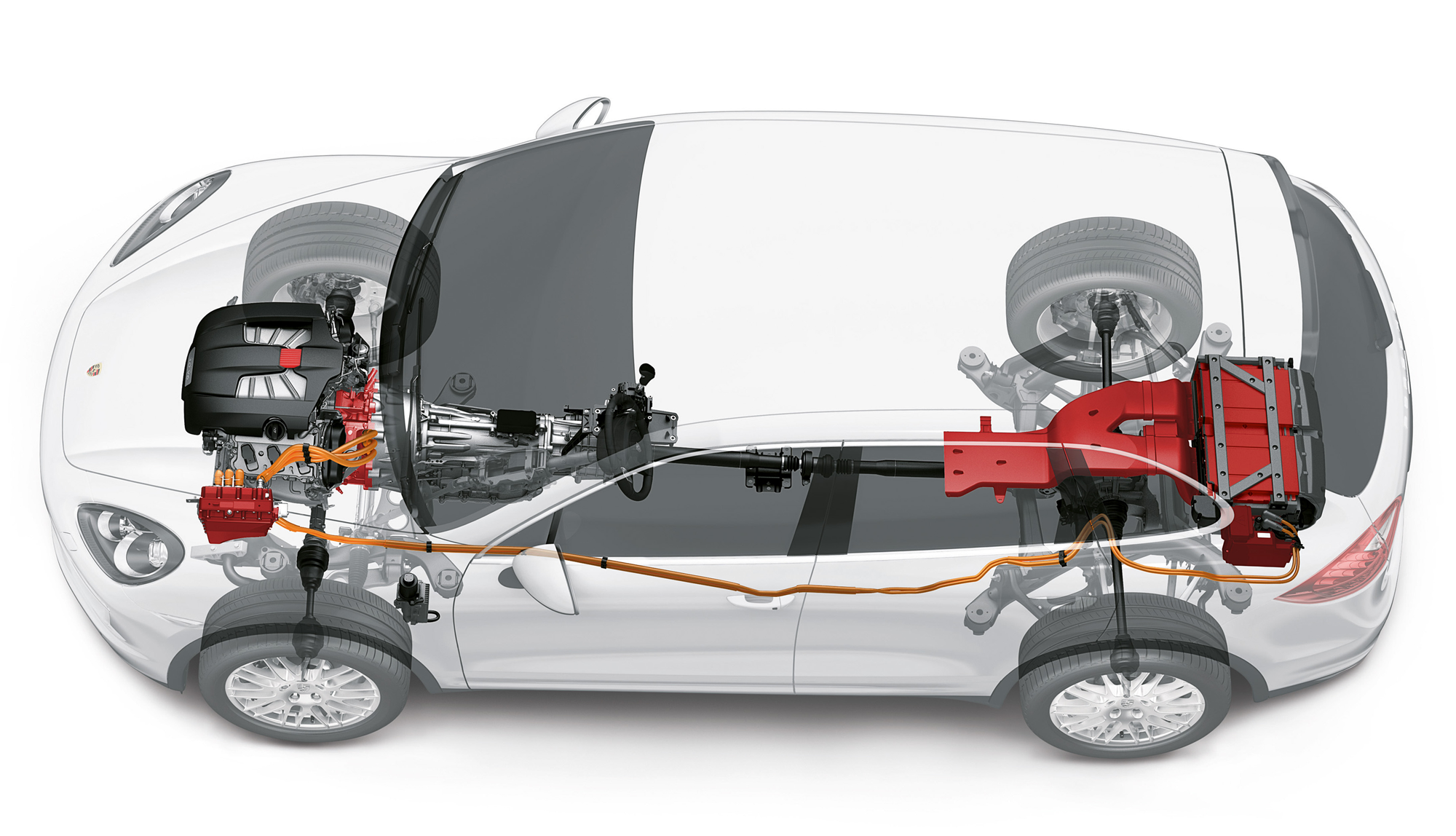
While working with modeling and simulations, I discovered Modelica, a language for developing simulation models. I worked extensively with Modelica, both during my Ph.D. as well as in my first job at Lawrence Berkeley National Laboratory. Modelica is a great tool for modeling cyber-physical systems, for example to study the fuel efficiency of an hybrid vehicle, or to evaluate the interactions between renewable energy sources and the electrical grid.

In this post I will provide a general overview on Modelica, and I’ll showcase some of its main features.

What is Modelica?

Modelica, as the name suggests, is a modeling language. Which type of models? Mathematical models. Modelica does not focus on a particular application domain, and gives you the freedom to model a variety of problems ranging from electro-mechanical systems for automotive or aerospace applications, to financial models for banks.

You can use the language to create mathematical models using any combination of the following formalisms

• differential equations
• algebraic equations
• difference equations
• discrete event systems

As you can imagine, this kind of flexibility makes it easier to tackle lots of different and interesting engineering problems, including cyber-physical systems. Typical examples of such systems are cars. Cars are characterized by mechanical components that interact with electronics and hydraulic systems, all under the supervision of multiple control systems. So if you want to know how a car is actually going to behave, you need to simulate the whole shebang.

Ignoring the interaction between components – a rookie mistake in the world of simulations – would lead to a poor understanding of the system.

It’s not hard to find other examples of cyber-phyisical systems, they’re everywhere you look:

• every private or public transportation vehicle – from airplanes to e-bikes
• the electrical grid that powers our houses
• data centers that process our data, etc.
• our homes, thanks to the increasing adoption of PV panels, batteries, EV cars, and IoT devices

So, at this point you should be convinced that cyber-physical systems are a big part of everyday life. Modelica allows engineers and scientists to model these systems accurately, giving us a chance to improve their performance. This is why Modelica matters.

Modeling the real world

Ask any engineer, and they’ll tell you - “It’s tough to model the real world!” Engineers perform a balancing act when they create models of complex physical systems, building detailed simulations while at the same time struggling against overwhelming complexity or irrelevant detail.

The Modelica modeling language has several features that make it the right choice for modeling complex engineering systems. Modelica is not some abstract academic toy disregarded by the modern industry. In fact, in the last few years Modelica has been adopted by some of the world’s biggest automotive companies – Audi, BMW, Daimler, Ford, Toyota, and VW. These companies use Modelica to design energy efficient vehicles, improve air conditioning systems. They Ferrari F1 team uses Modelica too for designing their racing cars! And the automotive sector is just one of many that find this language effective. The aerospace and energy industry are increasingly adopting Modelica, and the US Department of Energy has been steadily investing in this technology for modeling buildings and improving their energy efficiency.

Modelica - A first example

As described on the Modelica association website, Modelica is a non-proprietary, object-oriented, equation based language to conveniently model complex physical systems including a variety of different aspects, including mechanical, electrical, electronic, hydraulic, thermal, control, electric power or process-oriented subcomponents.

The following diagram shows the big picture behind any Modelica model

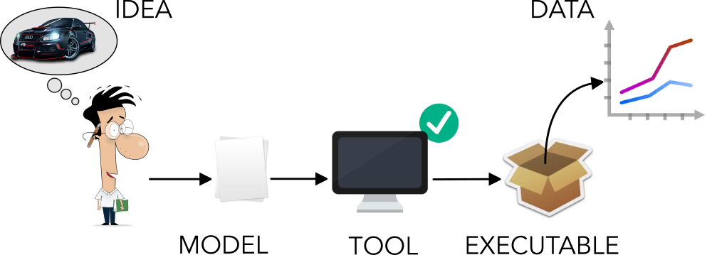
The steps are the following:

1. an engineer/scientist writes a Modelica model that represents an idea as a series of equations,
2. a Modelica tool analyzes the model and verifies its correctness – Does the model have the same number of variables and equations? Are there typos?
3. the tool compiles the model and generates an executable
4. run the executable to simulate the system and produce data.

Before diving into some of Modelica’s core concepts let’s start with an example, a kind of HelloWorld of differential equations. We’ll use the simplest differential equation you can imagine

with initial condition \( x(t_0) = 5 \)

 1 model HelloWorld  "The simplest differential equation ever"
 2   // Define variables and parameters here...
 3   Real x
 4     "The unknown variable";
 5   constant Real a = -2.0
 6     "Constant that characterizes the model";
 7   parameter Real x_start = 5.0
 8     "Initial value of the variable x";
 9 initial equation
10   // Define initial conditions here...
11   x = x_start;
12 equation
13   // Write the equations here...
14   der(x) = a*x;
15 end HelloWorld;

The keyword model defines the beginning of a model named HelloWorld. The model is divided in three sections: declarations, initializations and equations. The model starts by declaring variables, constants and parameters. Variables represent quantities that are expected to change over time. Constants, meanwhile, are fixed quantities that will never change. And finally parameters are quantities that do not change over time but may change between simulations. In this case parameter x_start, constant a and variable x have the same type, Real type meaning a floating point number.

The keywords initial equation introduce the second part of our model. Here we define the initial conditions of the system, for example the value of x at the beginning of our model’s simulation time.

The keyword equation introduces the third and final part of our program, where we finally get down to writing the equations of the system. In this case there is one variable x and one differential equation der(x) = a*x.

One important thing to note is the der(...) operator that indicates the time derivative of the expression inside the brackets. The ability to express derivatives in such a clean and concise way is very helpful when dealing with mathematical models.

Modelica’s key principles

So we’ve completed a simple example to get familiar with Modelica. Now, let’s look at some of its most interesting features. As I mentioned at the beginning of the post, Modelica is an object-oriented equation-based modeling language. What exactly do those words mean? Let’s have a look, keeping in the context of mathematical modeling.

Equation-based modeling

Computer programs are nothing but clever set of instructions to let a computer solve a particular problem for us (If this sounds familiar, bear with me. I’m going to make a distinction between assignments and equations that you might not be familiar with). Let’s consider the following problem: given two numbers compute their sum. The following code snippet shows a solution to the problem implemented in C

int main(void){
  int a, b, c;
  a = 4;
  b = 3;
  c = a + b;
  return 0;
}

What happens here when the program is executed is that the value 4 is inserted in the memory space associated to variable a, the value 3 is inserted in the memory space associated to variable b and then their sum is assigned to the memory space associated to variable c.

Given the initial problem, this program implements a particular solution to it. And, most of the time when we write algorithms we are writing specific solutions to certain problems. In this case the problem and its algorithmic solution were pretty straightforward!

Now here’s the kicker: when dealing with mathematical modeling the situation is quite different. You typically start with a set of equations that describe the general understanding of the system you want to model.

Then, you can collected data about that system, and feed it into those equations to start generating some interesting answers to your questions. Often there are multiple questions to answer, so the model should be as general as possible so that it can be be easily manipulated to answer all the questions.

Let’s get back to our problem: given two numbers compute their sum. The following is an example of a Modelica model that solves it

1 model Sum
2    Integer a, b, c;
3 equation
4    c - (a + b) = 0;
5    a = 4;
6    b - 3 = 0;
7 end Sum;

The content of line 4 is the essence of equation-based modeling. It all boils down to two concepts:

• c - (a + b) = 0 is an equation and equations are not assignment like the ones we’re used to write in C, Java, Python, etc.
• a = 4 and b - 3 = 0 are located on lines 5 and 6. Both lines come after the first equation, and because equations are not assignment, their order does not matter. The only thing that matters is that the model has the same number of variables and equations.

So it turns out that equation-based modeling is all about writing equations with code. The Modelica tool of choice will know how to symbolically analyze the model, extract equations, substitute variables in equations, sort them and apply the proper numerical methods to find the solution.

Working with Causality

The equation-based paradigm opens the door to an interesting concept called a-causality.

Before focusing on the meaning and implications of a-causality let’s have a look at an example based on Newton’s second law

The acceleration of an object as produced by a net force is directly proportional to the magnitude of the net force, in the same direction as the net force, and inversely proportional to the mass of the object.

Sir Isaac Newton

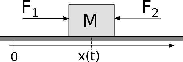
Newton’s second law describes a relationship between the following quantities: the forces acting on a body, the mass of the body and its acceleration.

The example below shows a system where a body that can move only along one direction and two forces are acting on it

Given this system, we can identify a number of problems to solve. Identifying a problem and finding its solution requires us follow a specific mental process:

• identify the known variables,
• rewrite Newton’s second law to find the desired quantity (e.g., acceleration, force, mass, etc.)

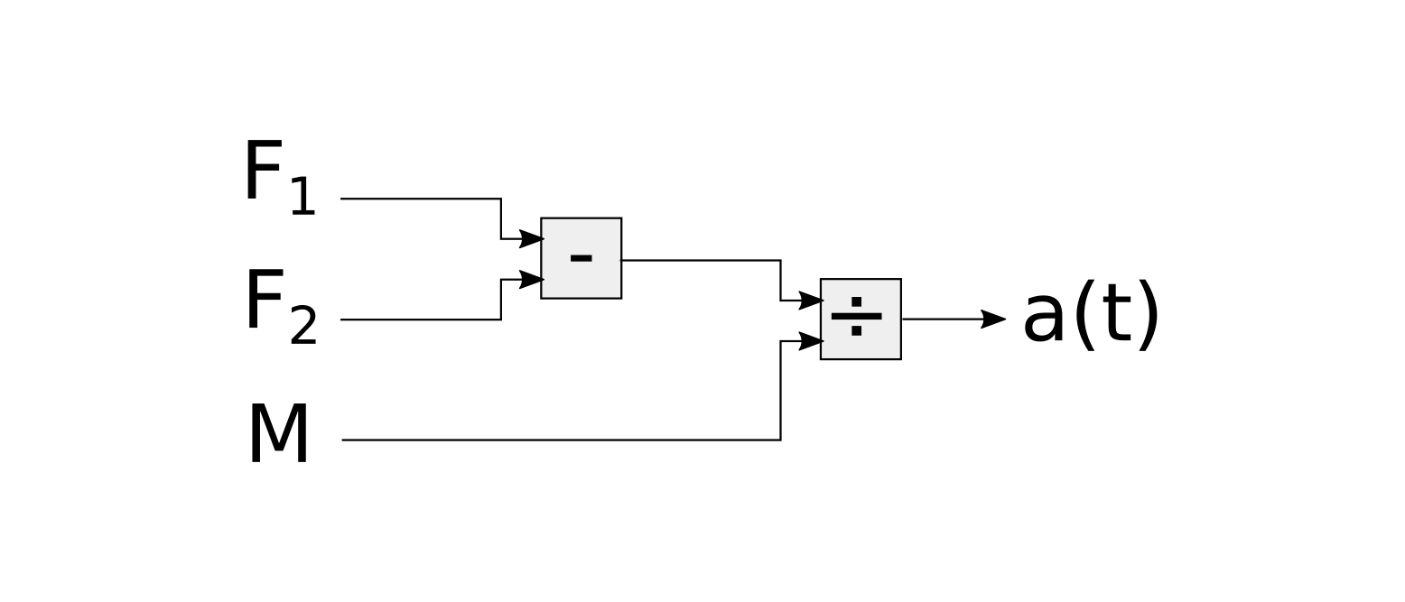
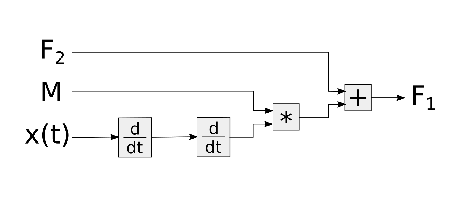
Here’s a small list of questions and their solutions presented with block diagrams; each diagram visually describes how the information flows from the inputs (i.e., known variables) to the output (i.e., answer to the question).

• given the mass, and the two forces compute the acceleration of the body

$$ a(t) =\frac{ F_1 - F_2}{M} $$

• given the mass, acceleration and one force compute the other force

$$ F_1 = F_2 + a(t) \, M$$

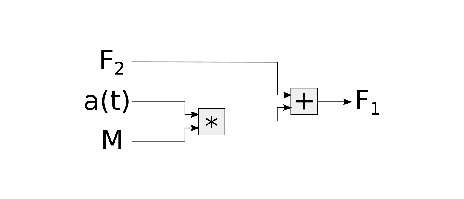
• given the two forces and the velocity of the body compute its mass

$$ M = \frac{F_1 - F_2}{\frac{d v(t)}{dt}} $$

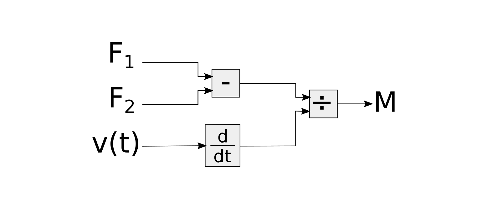
• given the position of the body, the mass, and one force compute the other force

$$ F_1 = F_2 + M \, \frac{d^2 \, x(t)}{dt^2}$$

This process requires a person that looks at the problem and

1. identifies relationships between the things that are known and the results to be found,
2. rearranges Newton’s second law in order to find a path that leads from one to the other.

What we’ve just seen is the so called causal approach: explicitly describe cause-effect relationships between variables and hard-code them in an algorithm that computes the solution. Even if the physical system is always the same, a slightly different question about the system might require a complete rewrite of the algorithm that solves the problem. The block diagrams above show this concept very well. Even if the underlying system is always the same, the type of operations performed on the data and the order of those operations changes continuously. This is rather inconvenient, especially when dealing with systems that are more complicated than a single body and a couple of forces!

Moreover, designing complex systems is an iterative process. New questions come up as the process evolves. Having an algorithm that can answer only one question and that needs to be rewritten to answer a slightly different one is not very useful.

Modelica’s equation-based nature enables the so called a-causal modelling approach: build mathematical models without imposing a priori cause-effect relationships between variables. Let’s try to model the same single body system in Modelica and see what it looks like.

 1 model SingleBodySystem
 2    Real M "The mass of the body";
 3    Real x "The position of the body";
 4    Real v "The velocity of the body";
 5    Real a "Acceleration of the body";
 6    Real F1, F2 "Forces acting on the body";
 7 initial equation
 8    // Initial conditions
 9    x = 0 "The position of the body is x=0 at time=0";
10    v = 0 "The body is not moving when time=0";
11 equation
12    // The dynamic behaviour of the system
13    v = der(x);
14    a = der(v);
15    M * a = F1 - F2;
16 
17    // Other "boundary" conditions
18    F1 = 1.2;
19    F2 = 2.0;
20    M  = 5.0;
21 end SingleBodySystem;

The equation section is divided in two parts. The first part describes Newton’s second law, i.e. the dynamic of the system. This part is not going to change unless the body starts moving at the speed of light!

The second part contains other “boundary” conditions. These conditions are required to have a complete picture of the system, and they can change from time to time depending on the question being asked.

When such conditions change the Modelica tool does all the hard work to finding causal relationships between the variables. Once the Modelica tools finds the relationships between inputs and outputs it generates an executable that solves the problem.

Such an approach leverages a computer for doing the boring and error prone job of rewriting and sorting equations. Computers are definitely better than humans at doing this!

A biproduct of a-causality is that models written in Modelica are more readable and maintainable. The model contains a description of the system and its boundary conditions rather than a solution to a specific problem. Most of the readers familiar with software engineering best practices know this is very important, especially when dealing with complex and large models.

After this brief discussion on a-causality I hope you’re convinced that writing ad-hoc solution to problems is similar to writing assembly code instead of using a higher level language and a compiler.

Variables and equations have units

As I already mentioned, Modelica variables can have types. Modelica gives the ability to associate units to variables. This feature is pretty simple but has a remarkable impact on the quality of the code. Adding units to variables/parameters/constants increases the ability to spot errors in the equations and makes the code more readable. What is more clear Real v or Modelica.SIunits.Volume v?!

The Modelica Standard Library (MSL available on Github) provides an extensive list of types that have units and extend the primitive type Real. This excerpt from the MSL shows how the ThermodynamicTemperature, Temperature, and SpecificHeatCapacity types are defined. Each type has a property called unit that is used to check the validty of the equations.

 1 type ThermodynamicTemperature = Real (
 2   final quantity="ThermodynamicTemperature",
 3   final unit="K",
 4   min = 0.0,
 5   start = 288.15,
 6   nominal = 300,
 7   displayUnit="degC"
 8 );
 9 
10 type Temperature = ThermodynamicTemperature;
11 
12 type SpecificHeatCapacity = Real (
13   final quantity="SpecificHeatCapacity",
14   final unit="J/(kg.K)"
15 );

Units can be simple like degrees Kelvin, denoted by the string K, or derived from others like the specific heat capacity, denoted by J/(kg.K), that is the energy per unit of mass that causes a temperature change of one degree Kelvin. The Modelica tool uses information about the type system and units to check if the models are valid or not. For example the following model

1 model TestSIUnits
2   Modelica.SIunits.Temperature T;
3   Modelica.SIunits.Energy E;
4   parameter Modelica.SIunits.SpecificHeatCapacity cp=1000;
5   parameter Modelica.SIunits.Mass m=1;
6 equation
7   T = 300;
8   E = cp*T; // Forgot to add m* ...
9 end TestSIUnits;

is not valid because the units in equation E = cp*T don’t match. The left side is energy and its unit is Joule J, the right side’s unit is Joule per Kelvin J/kg. When the tool parses and analyzes the model produces the following error Units error in equation E=cp*T, J != J/kg. Such an error message makes it pretty easy to understand that we forgot the mass, and the correct equation should have been E = m*cp*T.

Object-Oriented modeling

So far we’ve seen examples with few variables and simple equations. Real world systems are way more complicated than this. A-causality and types help keep the code more readabile and reduce bugs. This is just the tip of the iceberg, in order to model complex systems we need some extra features.

This is the where object-oriented modeling shines and where software engineering meets mathematical modeling.

The next example is this electric circuit, the series connection of a voltage source, a resistor and a capacitor (In case you’re not familiar with electrical circtuits bear with me, you’ll get the concepts anyway).

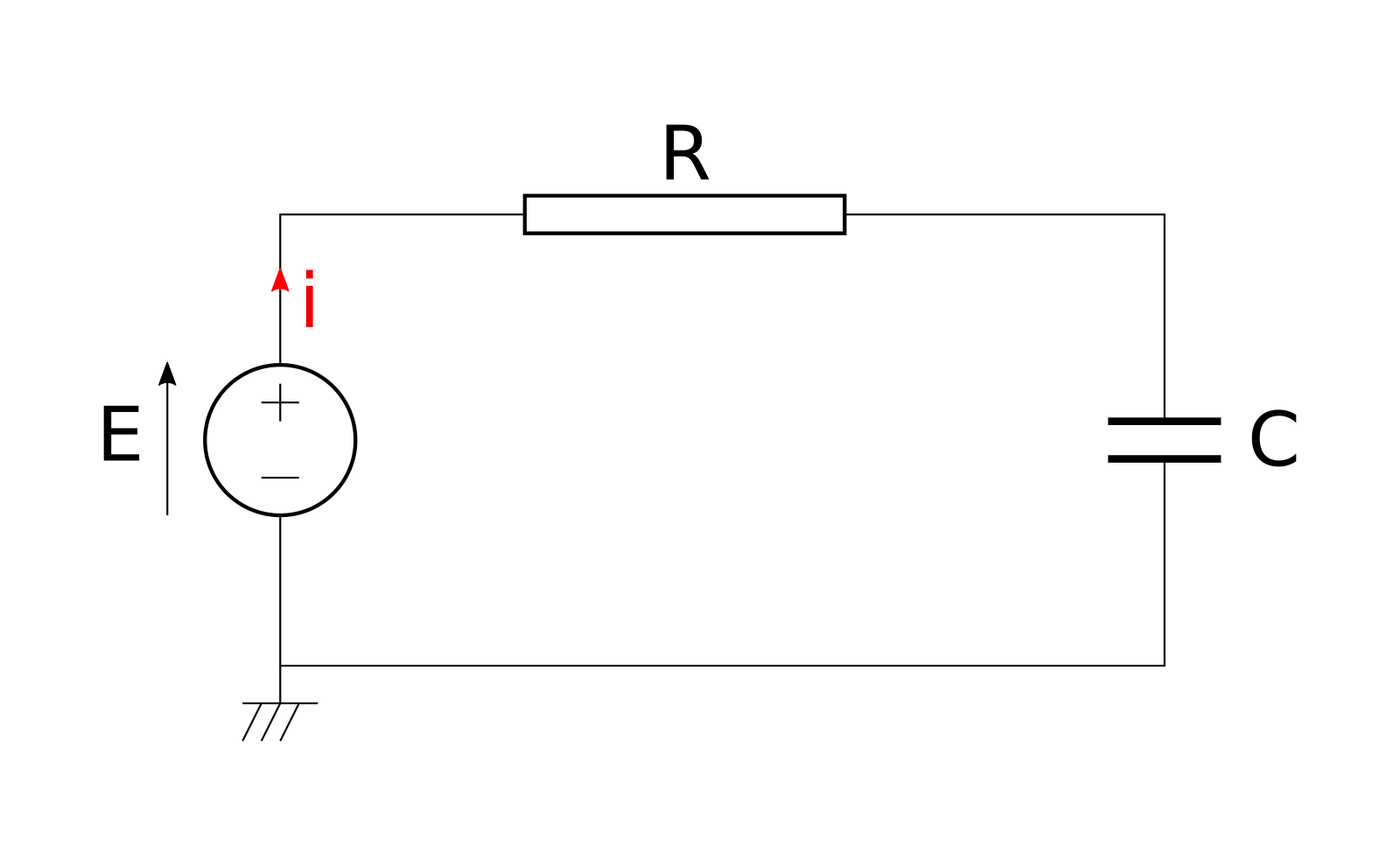
If we analyze the circuit using Kirchhof’s circuit laws we end up writing a Modelica model with the following equations

 1 model RC_v1 "RC model version 1.0"
 2   Modelica.SIunits.Voltage E
 3     "Voltage source";
 4   Modelica.SIunits.Voltage Vc
 5     "Voltage of the capacitor";
 6   Modelica.SIunits.Current i
 7     "Current flowing through the circuit";
 8   parameter Modelica.SIunits.Capacity C=1e-3
 9     "Capacity";
10   parameter Modelica.SIunits.Resistance R=1e3
11     "Resistance";
12 initial equation
13   Vc = 0.0;
14 equation
15   E = 10.0;
16   C*der(Vc) = i;
17   R*i = E - Vc;
18 end RC_v1;

The model represents the physical system in a “flat” way, there’s no clear distinction between the electrical components that are part of the circuit. We did not took advantage of the a-causality provided by Modelica and we ended up with a Model that represents this specific circuit.

It’s more convenient to imagine the circuit as a network of components that are connected to each other.

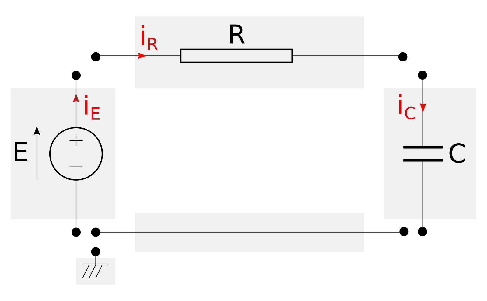
The image above shows an exploded view of the circuit and its components. Each component, enclosed in a grey rectangle, represents an actual piece of hardware (e.g., resistors, capacitors, cables, etc.).

Wouldn’t be better to have a library of virtual electric components that can be connected to generate all kinds of virtual circuits? Yes, and Modelica allows to create modular models that can be assembled like construction blocks thanks to connectors.

Connectors (aka Interfaces)

Modelica connectors are a construct that allows to connect models and let them exchange information. Connectors are inspired to real world physical interactions. Let’s have a look how actual electrical components work to gain some insight.

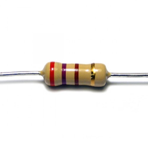
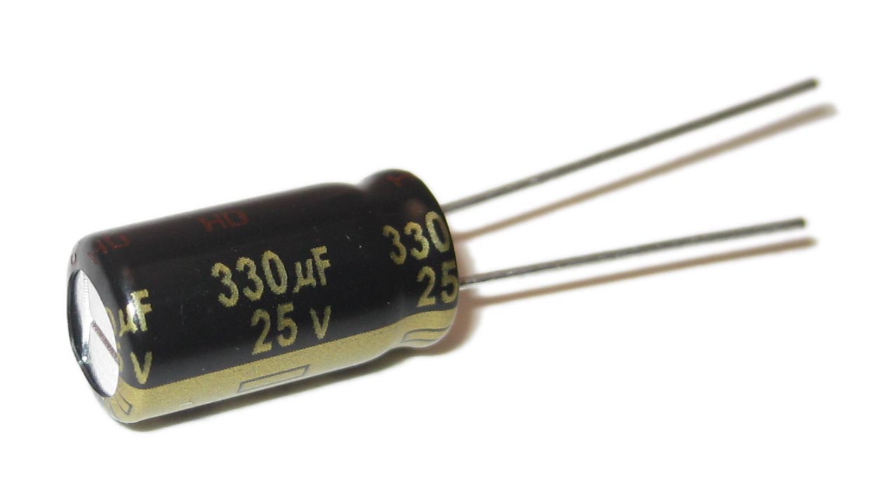
The pictures above show a resistor and a capacitor. They’re very different objects that behave according to different laws, however they share a common trait: they both have two wires (also known as terminal pins).

Resistors and capacitors don’t care in which part of the circuit are located, they behave in function of the voltages and currents provided to their terminals. Resistors and capacitors see the world through their terminals – and they work just fine.

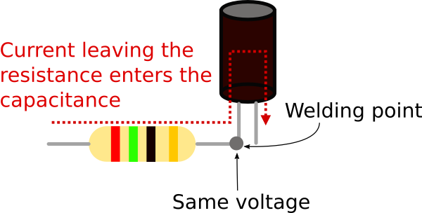
When an engineer designs a circuit in which resistors and capacitor interact with each other, their terminals are welded. Welding electric terminals imposes two physical constraints, the voltage at their junction becomes the same and the current leaving one component enters the other.

Modelica connectors are the equivalent of electic terminals as they define boundary conditions for models.

In the electrical domain the boundary conditions that characterize the behaviour of components such resistors or capacitors are voltages and currents. This means that a Modelica connector for electrical components will look like

1 connector Terminal "Connector/Interface for electrical systems"
2   Modelica.SIunits.Voltage v
3     "Voltage at the terminal";
4   flow Modelica.SIunits.Current i
5     "Current flowing through the terminal"
6     "(positive entering the model)";
7 end Terminal;

The connector defines two variables, the voltage v and the current i.

Connectors in Models

So far we’ve seen that connectors can be used to define boundary conditions. Now we’ll see how to use connectors for building a self contained model representing a resistor.

 1 model Resistor
 2   Terminal A, B;
 3   parameter Modelica.SIunits.Resistance R = 1e3
 4     "Resistance";
 5 equation
 6   // Constraint between connector variables
 7   // i.e. the current that enters
 8   // connector A leaves connector B
 9   A.i + B.i = 0;
10 
11   // Ohm's law
12   A.v - B.v = R*A.i;
13 end Resistor;

The model has two electrical terminals A, B, and a parameter R (the value of the resistance). The equations describe the behaviour of the component based on the boundary conditions provided by the connectors.

Equation A.v - B.v = R*A.i states that the voltage difference between terminal A and B is equal to the current entering from terminal A multiplied by the resistance R.

Equation A.i + B.i = 0 states that the current entering from terminal A plus the current entering from therminal B is equal to zero – i.e. the current entering from A leaves from B (please note that currents are always measured as positive when entering the model).

In a similar way we can build component models for all of the remaining elements: source, capacitor and ground reference.

 1 model Source
 2   Terminal A, B;
 3   parameter Modelica.SIunits.Voltage E = 10
 4     "Constant voltage source";
 5 equation
 6   // Constraint between connector variables
 7   // i.e. the same amount of current that enters from
 8   // connector A leaves from connector B
 9   A.i + B.i = 0;
10 
11   // The source generates a voltage difference
12   // between the two terminals
13   A.v - B.v = E;
14 end Source;
15 
16 model Capacitor
17   Terminal A, B;
18   parameter Modelica.SIunits.Capacitance C = 1e-3
19     "Capacitance";
20   parameter ModelicA.SIunits.Voltage Vc_start = 0.0
21     "Initial voltage of the capacitor";
22   Modelica.SIunits.Voltage Vc;
23 initial equation
24   Vc = Vc_start;
25 equation
26   // Constraint between connector variables
27   // i.e. the same amount of current that enters from
28   // connector A leaves from connector B
29   A.i + B.i = 0;
30 
31   // Change in the charge is equal to the current flow
32   C*der(Vc) = A.i;
33   Vc = A.v - B.v;
34 
35 end Capacitor;
36 
37 model Ground
38   Terminal A;
39 equation
40   // Boundary condition that fixes the voltage reference
41   A.v = 0.0;
42 end Ground;

Connecting Models

At this point we have defined models of all the electrical components we need. Each component has terminals and in order to build a circuit we have to connect them. Modelica has a construct called connect(.,.) and it’s purpose is to connect connectors.

This is the new version of the Modelica model that represents the circuit.

 1 model RC_v2 "RC model version 2.0"
 2   Source S(E=10)  "Voltage source";
 3   Capacitor C(Vc_start=0.0, C=1e-3) "Capacitor";
 4   Resistor R(R=1e3) "Resistance";
 5   Ground ref "Ground reference";
 6 equation
 7   connect(S.A, R.A);
 8   connect(S.B, ref.A);
 9   connect(R.B, C.A);
10   connect(C.B, ref.A);
11 end RC_v2;

This version of the model that uses components and connectors is more readable than the flat representation we started with. The first part of the model defines all the components we’re using while the second part defines how they are connected. Nedless to say that this model is more maintainable than the previous “flat” version. Modularity and reusability improve as well because each component can be replaced and they are ready to be reused in other circuits without any effort.

Connect’s magic

The model we just wrote is very readable but what happened to all the equations we used to write? And why is the connect statement included in the equation section?

Every time we connect two connectors with a connect(., .) operator the Modelica tool that analyzes the code adds some equations for us. The equations that are automatically added impose the constraints that are enforced when welding terminal pins in the real world

1. voltages become equal,
2. the current leaving one terminal enters the other.

The image below shows two Terminal connectors named A and B and the equations that are generated when they’re connected.

Again, less tedious work for us to do and less opportunities to introduce errors.

Partial models = abstract classes

At this point the software engineer in the room should stop me and tell everyone “This is good, but I think we can do better than this”.

Creating mathematical models in Modelica (or Matlab, or whatever you like) is still software development. Software engineering practices and well understood design patterns should be leveraged when writing mathematical models.

This is particularly true for people who design Modelica libraries that are used by many and contain houndreds of components. The pleople who design these libraries must have in mind a clear vision on how the library should be structured, which connectors are needed, etc.

The createators of Modelica knew about SW engineering, and they baked into the language several features that are mostly inspired to Object-Oriented programming. One of the most useful features is the ability to create partial models.

For example Source, Resistor, and Capacitor share quite a bit of code. Each model defines the connectors A and B as well the equation A.i + B.i = 0. This is against the DRY principle and fortunately there’s a simple solution: partial models.

Partial models are models that allows to declare variables, parameters, and equations but don’t have to be complete. This means that a partial model can have more variables than equations. The missing equations will be provided by models that extend the partial model. In case you’re familiar with OO programming, partial models are the Modelica version of abstract classes. Let’s see how the models created so far can be refactored using this feature

The first step is to isolate the traits (parameters, connectors, equations, etc.) shared by multiple models and collect them into a partial model. In this case the partial model represents a bipole, i.e. a generic electric component with two terminals where the sum of the currents entering and leaving is zero.

 1 partial model Bipole "Electrical model with two pins"
 2   Terminal a, b;
 3   Modelica.SIunits.Voltage V
 4     "Voltage drop";
 5   Modelica.SIunits.current i
 6     "Current entering terminal a";
 7 equation
 8   // Constraint between connector variables
 9   // i.e. the same amount of current that enters from
10   // connector a leaves from connector b
11   A.i + B.i = 0;
12 
13   // Definition of utility variables
14   V = A.v - B.v;
15   i = A.i;
16 
17 end Bipole;

The resistor, capacitor and source now become extensions of this basic model.

 1 model Resistor
 2   extends Bipole;
 3   parameter Modelica.SIunits.Resistance R = 1e3
 4     "Resistance";
 5 equation
 6   // Ohm's law
 7   V = R*i;
 8 end Resistor;
 9 
10 model Source
11   extends Bipole;
12   parameter Modelica.SIunits.Voltage E = 10
13     "Constant voltage source";
14 equation
15   // The source generates a voltage difference
16   // between the two terminals
17   V = E;
18 end Source;
19 
20 model Capacitor
21   extends Bipole;
22   parameter Modelica.SIunits.Capacitance C = 1e-3
23     "Capacitance";
24   parameter Modelica.SIunits.Voltage V_start = 0.0
25     "Initial voltage of the capacitor";
26 initial equation
27   V = V_start;
28 equation
29   // Change in the charge is equal to the current flow
30   C*der(V) = i;
31 end Capacitor;

Again, readability and maintenability increases. Plus, if now we wish to create a new model for an inductor or a variable resistor there already is a partial model to extend that declares the basic structure.

Conclusions

So, if you’ve made it this far, you should be convinced that cyber-physical systems are a big part of everyday life, and Modelica helps engineers and scientists to model these systems accurately.

There’s a lot to be said about Modelica, and in this post we just scratched the surface. We have seen that Modelica works directly with equations and that this leads to a-causal models. We also learned that a-causal models are more readable and flexible, making then a good way to express complex engineering problems. We also learned about some of the language features inspired by SW engineering: typed variables and object-oriented features that promote encapsulation.

If after reading this post you’re even more interested in Modelica I suggest you to look at the online book Modelica by examples by Michael Tiller, otherwise browse the website of the Modelica associations www.modelica.org. Here you can freely access houndreds of papers that have been written over the years and presented during the numerous Modelica conferences around the world.

If you’re interested in the work I’ve done with Modelica, you can look here.

Aknowledgments

Special thanks to Daniel McQuillen for proof reading this post and providing helpful suggestions, and to Daniel Gackle for suggesting to combine my previous articles on this topic into a single one.

Back to POSTS