Modelica in action: compile and simulate models
by Marco Bonvini on Monday January 02, 2017
In the last posts I explained why Modelica matters and some of the features that make Modelica a great language for modeling dynamic systems. In this post I focus on some practical aspects, namely how to setup the open-source JModelica platform and how to compile and simulate Modelica models. The post is accompanied by a Github repository called ModelicaInAction. This repository contains all the code and the instructions needed to setup JModelica and running the examples.
Modelica is a non-proprietary, object-oriented, equation based language to conveniently model complex physical systems. In order to compile and simulate Modelica models you need a simulation environment. The Modelica association website provides a list of the comercial and open source Modelica simulation environments.
In this demo I use JModelica.org, an extensible Modelica-based open source platform for optimization, simulation and analysis of complex dynamic systems.
Installing JModelica
Installing JModelica is a lengthy process because it depends on many external and third party packages. To ease the installation process I created a Docker container with installed everything that is needed to run the examples.
In case you wonder what’s a Docker container
Docker containers wrap a piece of software in a complete filesystem that contains everything needed to run: code, runtime, system tools, system libraries – anything that can be installed on a server. This guarantees that the software will always run the same, regardless of its environment (see https://www.docker.com/what-docker for more info).
In this case I created a “recipe”, also known as Docker file, that describes how to build a container with installed everything that’s needed to start using JModelica.
Once created and started, the container and your OS will interact as shown in the following image.
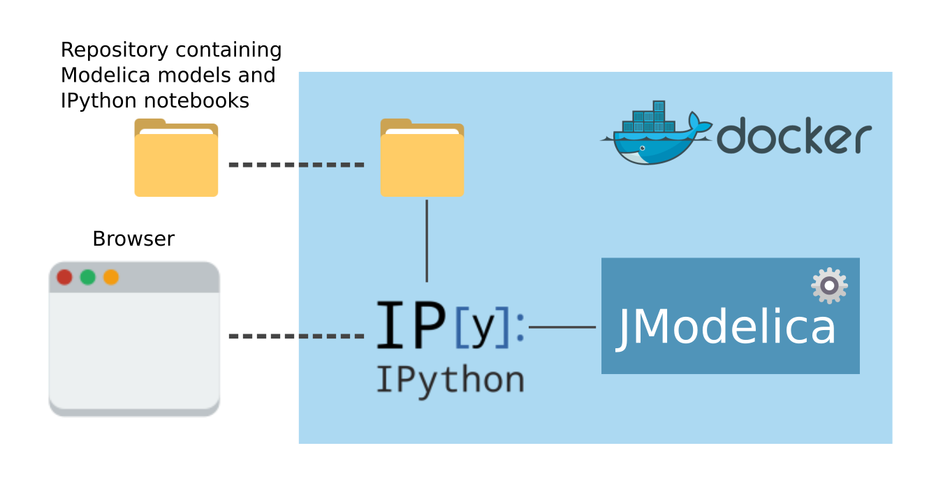
Upon start, some folders included in the repository ModelicaInAction will be shared with the container, in the meantime the container runs an IPython server and exposes the port where it listens to your local machine. In this way you can connect to the IPython server running inside the container with a browser.
Once you connect to the IPython server that is available at localhost:8888 you should see something like this
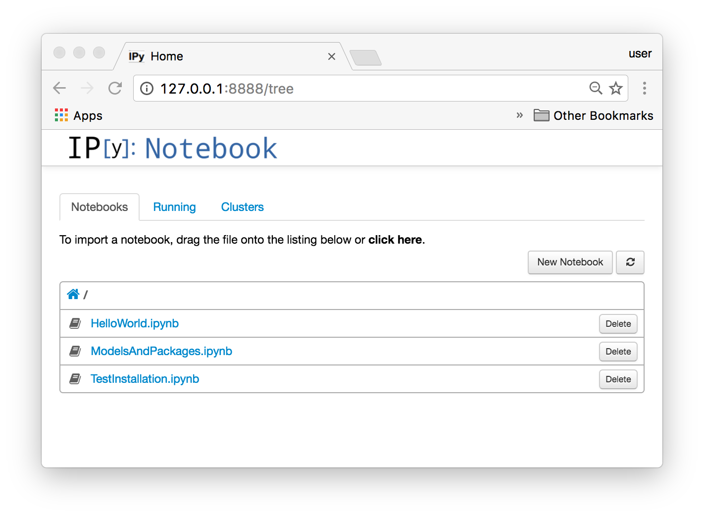
Each IPython notebook contains an example that is covered by one of my posts. For example in the following section we will see how to compile and simulate a Modelica model that is covered by the notebook HelloWorld.ipynb.
For a detailed explanation on how to download and start the Docker container please refer to the README.md file on Github.
Compile and simulate a model
In this first example we will learn how to compile and simulate a model. To keep the complexity as low as possible we’re going to simulate the HelloWorld model I introduced in this post about Modelica basics.
The model to simulate is defined in a file called HelloWorld.mo that is located in
the modelica folder that is part
of the ModelicaInAction repository.
The content of the file is the following
 1 // Content of file ModelicaInAction/modelica/HelloWorld.mo
 2
 3 model HelloWorld  "The simplest differential equation ever"
 4   // Define variables and parameters here...
 5   Real x
 6     "The unknown variable";
 7   constant Real a = -2.0
 8     "Constant that characterizes the model";
 9   parameter Real x_start = 5.0
10     "Initial value of the variable x";
11 initial equation
12   // Define initial conditions here...
13   x = x_start;
14 equation
15   // Write the equations here...
16   der(x) = a*x;
17 end HelloWorld;
This files, as well the other files contained in the folder [...]/ModelicaInAction/modelica are shared
with the Docker container. In particular the folder is attached to the folder /home/docker/modelica
inside the container. This means that when we’ll use JModelica from the IPython notebook we can
reference this file as /home/docker/modelica/HelloWorld.mo.
To compile the model we use the following instructions
1 from pymodelica import compile_fmu
2
3 # Specify Modelica model and model file (.mo or .mop)
4 model_name = 'HelloWorld'
5 mo_file = '/home/docker/modelica/HelloWorld.mo'
6
7 # Compile the model and save the return argument,
8 # which is the file name of the FMU
9 my_fmu = compile_fmu(model_name, mo_file)
The function compile_fmu(...) in its simplest form takes two parameters,
the name of the model to compile and the name of the file that contains the
definition of the model. The function opens the file, parses the model, analyzes the
equations and it generates a binary file that can be used to simulate the model.
The binary file createed by JModelica is an FMU (Functional Mockup Unit). An FMU is a file compliant with the Functional Mock-up Interface (FMI). FMI is a tool independent standard to support both model exchange and co-simulation of dynamic models using a combination of xml-files and compiled C-code.
TL;DR, JModelica generates C-code that is boundled together with an xml representation of the model. Both the C-code and the xml-files are packaged inside the FMU.
The next step is to take this FMU and run a simulation.
1 from pyfmi import load_fmu
2 from matplotlib import pyplot as plt
3
4 # Load the model and simulate
5 hello_world = load_fmu(my_fmu)
6 res = hello_world.simulate(final_time=5.0)
7
8 # Plot the results
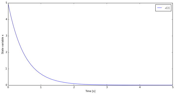
9 plt.plot(res["time"], res['x'], label="$x(t)$")
10 plt.xlabel("Time [s]")
11 plt.ylabel("State variable x")
12 plt.legend()The function load_fmu(...) loads the FMU and returns an object that
represents a generic simulation model. Such simulation model object has many
methods and one of them is simulate(...).
The simulate method links the C-code representing the model to
numerical ODE integrators such as CVode (or others solver that are part of
Sundials) and runs a simulation.
The simulate(...) method returns a result object containing the values of the variables
in a dictionary-like structure. In this case we plot the value of the state variable
x versus time.
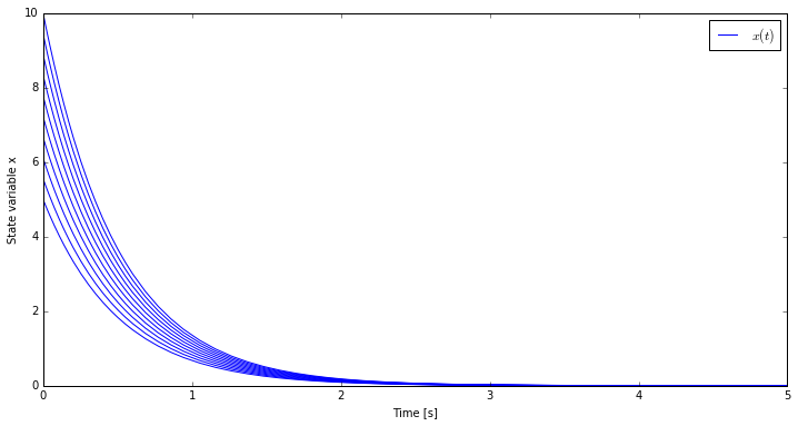
We can do more that simply simulating the model, for example we can re-simulate our model starting
from tens of different initial conditions. If we take a look at the model we can see that there is
a parameter x_init, that is the value assumed by the state variable x at the beginning of the simulation.
Therefore, to simulate the model from multiple initial conditions we have to change the value of
x_init.
The following code snippet shows how to simulate
the model for multiple values of the parameter x_init and saving the result of each simulation.
A small note, because the model has already been simulated to run a new simulation we need to reset the model.
To reset the model we use the reset() method.
1 import numpy as np
2
3 x_init = np.linspace(5.0, 10.0, 10)
4 results = []
5 for xi in x_init:
6     hello_world.reset()
7     hello_world.set("x_start", xi)
8     results.append(hello_world.simulate(final_time=5.0))
The result of these simulations can be plotted and as expected even if the
state variable x starts from different initial conditions it always
converges to zero in the same time.
Conclusions
After describing all the nice features provided by Modelica, in this post we finally compiled and simulated our first model!
I also introduced this new repository ModelicaInAction. The purpose of this repository is to provide the readers an environment where they can test and run the models and examples described in my posts.
We just scratched the surface of what can be done with JModelica. In the following post I will show you an other pratical tip: how to organize models in packages.