SW engineering meets mathematical modeling - Types and Objects
by Marco Bonvini on Sunday October 23, 2016
This post is the second of a series of posts that cover some of the most important features provided by Modelica. Here I’ll describes the type system used by Modelica and how it helps avoiding trivial errors when writing equations. The post continues with a description of the Object-Oriented features provided by Modelica and how they help engineers model complex systems in a modular way.
Variables and equations have units
When in the previous post, SW engineering meets mathematical modeling - Modelica basics,
I said that Modelica variables have types the story wasn’t complete. Modelica gives the ability to
associate units to variables. This feature is pretty simple but has a remarkable impact on the quality
of the code. Adding units to variables/parameters/constants increases the ability to spot
errors in the equations and makes the code more readable.
What is more clear Real v or Modelica.SIunits.Volume v?!
The Modelica Standard Library (MSL available on Github) provides an
extensive list of types that have units and extend the primitive type Real. This excerpt from the MSL shows
how the ThermodynamicTemperature, Temperature, and SpecificHeatCapacity types are defined.
Each type has a property called unit that is used to check the validty of the equations.
 1 type ThermodynamicTemperature = Real (
 2   final quantity="ThermodynamicTemperature",
 3   final unit="K",
 4   min = 0.0,
 5   start = 288.15,
 6   nominal = 300,
 7   displayUnit="degC"
 8 );
 9
10 type Temperature = ThermodynamicTemperature;
11
12 type SpecificHeatCapacity = Real (
13   final quantity="SpecificHeatCapacity",
14   final unit="J/(kg.K)"
15 );
Units can be simple like degrees Kelvin, denoted by the string K, or
derived from others like the specific heat capacity,
denoted by J/(kg.K), that is the energy per unit of mass that causes a temperature change of one degree Kelvin.
The Modelica tool uses information about the type system and units to
check if the models are valid or not. For example the following model
1 model TestSIUnits
2   Modelica.SIunits.Temperature T;
3   Modelica.SIunits.Energy E;
4   parameter Modelica.SIunits.SpecificHeatCapacity cp=1000;
5   parameter Modelica.SIunits.Mass m=1;
6 equation
7   T = 300;
8   E = cp*T; // Forgot to add m* ...
9 end TestSIUnits;
is not valid because the units in equation E = cp*T don’t match. The left side is energy
and its unit is Joule J, the right side’s unit is Joule per Kelvin J/kg. When the tool
parses and analyzes the model produces the following error
Units error in equation E=cp*T, J != J/kg. Such an error message makes it pretty easy to
understand that we forgot the mass from the correct equation E = m*cp*T.
Object-Oriented modeling
So far we’ve seen examples with few variables and simple equations. Real world systems are way more complicated than this. A-causality and types help keep the code more readabile and reduce bugs. This is just the tip of the iceberg, in order to model complex systems we need some extra features.
This is the where Object-Oriented modeling shines and where software engineering meets mathematical modeling.
The next example is this electric circuit, the series connection of a voltage source, a resistor and a capacitor (In case you’re not familiar with electrical circtuits bear with me, you’ll get the concepts anyway).
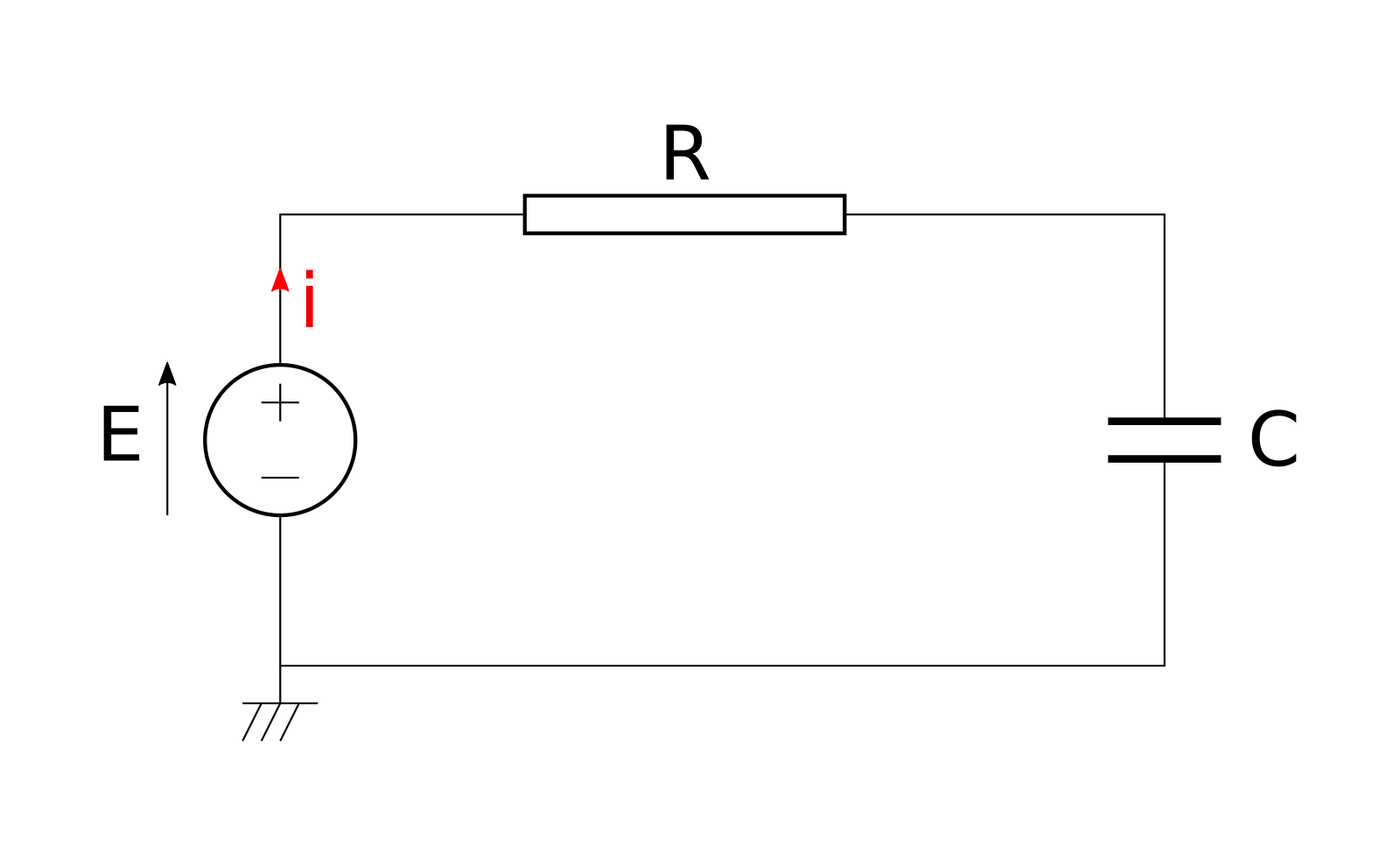
If we analyze the circuit using Kirchhof’s circuit laws we end up writing the following Modelica model
 1 model RC_v1 "RC model version 1.0"
 2   Modelica.SIunits.Voltage E
 3     "Voltage source";
 4   Modelica.SIunits.Voltage Vc
 5     "Voltage of the capacitor";
 6   Modelica.SIunits.Current i
 7     "Current flowing through the circuit";
 8   parameter Modelica.SIunits.Capacity C=1e-3
 9     "Capacity";
10   parameter Modelica.SIunits.Resistance R=1e3
11     "Resistance";
12 initial equation
13   Vc = 0.0;
14 equation
15   E = 10.0;
16   C*der(Vc) = i;
17   R*i = E - Vc;
18 end RC_v1;
The model represents the physical system in a “flat” way, there’s no clear distinction between the electrical components that are part of the circuit. We did not took advantage of the a-causality provided by Modelica and we ended up with a Model that represents this specific circuit.
It’s more convenient to imagine the circuit as a network of components that are connected to each other.
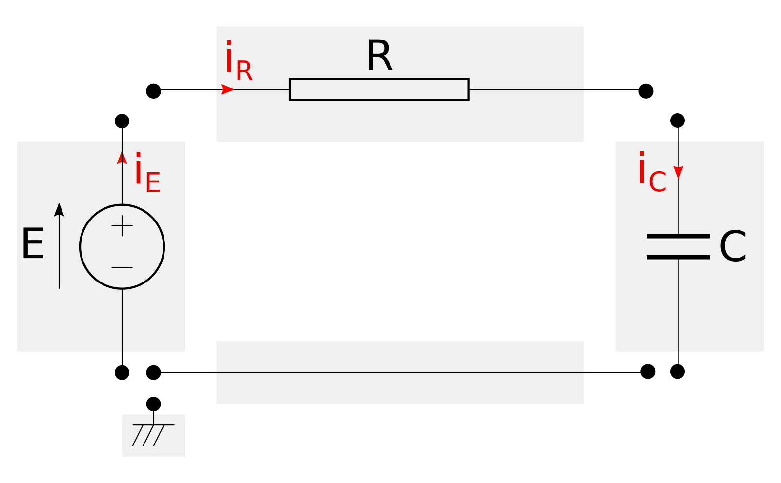
The image above shows an exploded view of the circuit and its components. Each component, enclosed in a grey rectangle, represents an actual piece of hardware (e.g., resistors, capacitors, cables, etc.).
Wouldn’t be better to have a library of virtual electric components that can be connected to generate all kinds of virtual circuits? Yes, and Modelica allows to create modular models that can be assembled like construction blocks thanks to the so called connectors.
Connectors (aka Interfaces)
Modelica connectors are a construct that allows to connect models and let them exchange information. Connectors are inspired to real world physical interactions. Let’s have a look how actual electrical components work to gain some insight.
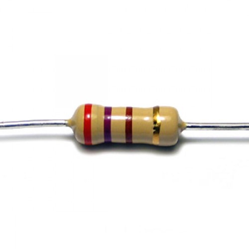
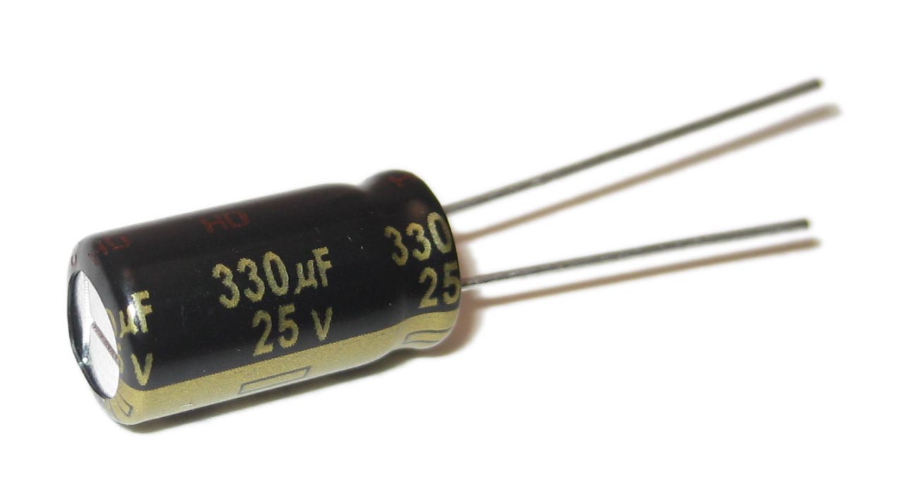
The pictures above show a resistor and a capacitor. They’re very different objects that behave according to different laws, however they share a common trait: they both have two wires (also known as terminal pins).
Resistors and capacitors don’t care in which part of the circuit are located, they behave in function of the voltages and currents provided to their terminals. Resistors and capacitors see the world through their terminals – and they work just fine.
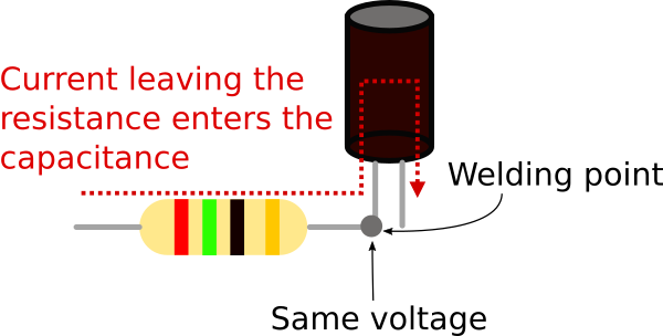
When an engineer designs a circuit in which resistors and capacitor interact with each other, their terminals are welded. Welding electric terminals imposes two physical constraints, the voltage at their junction becomes the same and the current leaving one component enters the other.
Modelica connectors are the equivalent of electic terminals as they define boundary conditions for models.
In the electrical domain the boundary conditions that characterize the behaviour of components such resistors or capacitors are voltages and currents. This means that a Modelica connector for electrical components will look like
1 connector Terminal "Connector/Interface for electrical systems"
2   Modelica.SIunits.Voltage v
3     "Voltage at the terminal";
4   flow Modelica.SIunits.Current i
5     "Current flowing through the terminal"
6     "(positive entering the model)";
7 end Terminal;
The connector defines two variables, the voltage v and the current i.
Connectors in Models
So far we’ve seen that connectors can be used to define boundary conditions. Now we’ll see how to use connectors for building a self contained model representing a resistor.
 1 model Resistor
 2   Terminal A, B;
 3   parameter Modelica.SIunits.Resistance R = 1e3
 4     "Resistance";
 5 equation
 6   // Constraint between connector variables
 7   // i.e. the current that enters
 8   // connector A leaves connector B
 9   A.i + B.i = 0;
10
11   // Ohm's law
12   A.v - B.v = R*A.i;
13 end Resistor;
The model has two electrical terminals A, B, and a parameter R (the value of the resistance).
The equations describe the behaviour of the component based on the boundary conditions provided by the
connectors.
Equation A.v - B.v = R*A.i states that the voltage difference between terminal A and B
is equal to the current entering from terminal A multiplied by the resistance R.
Equation A.i + B.i = 0 states that the current entering from terminal A plus the current
entering from therminal B is equal to zero – i.e. the current entering from A leaves from B
(please note that currents are always measured as positive when entering the model).
In a similar way we can build component models for all of the remaining elements: source, capacitor and ground reference.
 1 model Source
 2   Terminal A, B;
 3   parameter Modelica.SIunits.Voltage E = 10
 4     "Constant voltage source";
 5 equation
 6   // Constraint between connector variables
 7   // i.e. the same amount of current that enters from
 8   // connector A leaves from connector B
 9   A.i + B.i = 0;
10
11   // The source generates a voltage difference
12   // between the two terminals
13   A.v - B.v = E;
14 end Source;
15
16 model Capacitor
17   Terminal A, B;
18   parameter Modelica.SIunits.Capacitance C = 1e-3
19     "Capacitance";
20   parameter ModelicA.SIunits.Voltage Vc_start = 0.0
21     "Initial voltage of the capacitor";
22   Modelica.SIunits.Voltage Vc;
23 initial equation
24   Vc = Vc_start;
25 equation
26   // Constraint between connector variables
27   // i.e. the same amount of current that enters from
28   // connector A leaves from connector B
29   A.i + B.i = 0;
30
31   // Change in the charge is equal to the current flow
32   C*der(Vc) = A.i;
33   Vc = A.v - B.v;
34
35 end Capacitor;
36
37 model Ground
38   Terminal A;
39 equation
40   // Boundary condition that fixes the voltage reference
41   A.v = 0.0;
42 end Ground;
Connecting Models
At this point we have defined models of all the electrical components we need. Each
component has terminals and in order to build a circuit we have to connect them.
Modelica has a construct called connect(.,.) and it’s purpose is to connect connectors.
This is the new version of the Modelica model that represents the circuit.
 1 model RC_v2 "RC model version 2.0"
 2   Source S(E=10)  "Voltage source";
 3   Capacitor C(Vc_start=0.0, C=1e-3) "Capacitor";
 4   Resistor R(R=1e3) "Resistance";
 5   Ground ref "Ground reference";
 6 equation
 7   connect(S.A, R.A);
 8   connect(S.B, ref.A);
 9   connect(R.B, C.A);
10   connect(C.B, ref.A);
11 end RC_v2;
This version of the model that uses components and connectors is more readable than the flat representation we started with. The first part of the model defines all the components we’re using while the second part defines how they are connected. Nedless to say that this model is more maintainable than the previous “flat” version. Modularity and reusability improve as well because each component can be replaced and they are ready to be reused in other circuits without any effort.
Connect’s magic
The model we just wrote is very readable but what happened to all the equations we used to write? And why is the connect statement included in the equation section?
Every time we connect two connectors with a connect(., .) operator under the hood
the Modelica tool that analyzes the code adds some equations for us.
The equations that are automatically added impose the constraints
that are enforced when welding terminal pins in the real world
- voltages become equal,
- the current leaving one terminal enters the other.
The image below shows two Terminal connectors named A and B and the equations that are
generated when they’re connected.

Again, less tedious work for us to do and less opportunities to introduce errors.
Partial models = abstract classes
At this point the software engineer in the room should stop me and tell everyone “This is good, but I think we can do better than this”.
Creating mathematical models in Modelica (or Matlab, or whatever you like) is still software development. Software engineering practices and well understood design patterns should be leveraged when writing mathematical models.
This is particularly true for people who design Modelica libraries that are used by many and contain houndreds of components. The pleople who design these libraries must have in mind a clear vision on how the library should be structured, which connectors are needed, etc.
The guys who created Modelica know this and they baked into the language several features that are mostly inspired to Object-Oriented programming. One of the most useful features is the ability to create partial models.
For example Source, Resistor, and Capacitor share quite a bit of code.
Each model defines the connectors A and B as well the equation A.i + B.i = 0.
This is against the DRY principle and fortunately
there’s a simple solution: partial models.
Partial models are models that allows to declare variables, parameters, and equations but don’t have to be complete. This means that a partial model can have more variables than equations. The missing equations will be provided by models that extend the partial model. In case you’re familiar with OO programming, partial models are the Modelica version of abstract classes. Let’s see how the models created so far can be refactored using this feature
The first step is to isolate the traits (parameters, connectors, equations, etc.) shared by
multiple models and collect them into a partial model. In this case the partial model
represents a bipole, i.e. a generic electric component with two terminals where the sum of
the currents entering and leaving is zero.
 1 partial model Bipole "Electrical model with two pins"
 2   Terminal a, b;
 3   Modelica.SIunits.Voltage V
 4     "Voltage drop";
 5   Modelica.SIunits.current i
 6     "Current entering terminal a";
 7 equation
 8   // Constraint between connector variables
 9   // i.e. the same amount of current that enters from
10   // connector a leaves from connector b
11   A.i + B.i = 0;
12
13   // Definition of utility variables
14   V = A.v - B.v;
15   i = A.i;
16
17 end Bipole;
The resistor, capacitor and source now become extensions of this basic model.
 1 model Resistor
 2   extends Bipole;
 3   parameter Modelica.SIunits.Resistance R = 1e3
 4     "Resistance";
 5 equation
 6   // Ohm's law
 7   V = R*i;
 8 end Resistor;
 9
10 model Source
11   extends Bipole;
12   parameter Modelica.SIunits.Voltage E = 10
13     "Constant voltage source";
14 equation
15   // The source generates a voltage difference
16   // between the two terminals
17   V = E;
18 end Source;
19
20 model Capacitor
21   extends Bipole;
22   parameter Modelica.SIunits.Capacitance C = 1e-3
23     "Capacitance";
24   parameter Modelica.SIunits.Voltage V_start = 0.0
25     "Initial voltage of the capacitor";
26 initial equation
27   V = V_start;
28 equation
29   // Change in the charge is equal to the current flow
30   C*der(V) = i;
31 end Capacitor;
Again, readability and maintenability increases. Plus, if now we wish to create a new model for an inductor or a variable resistor there already is a partial model to extend that declares the basic structure.
Conclusions
In this post I walked you through two other important features provided by Modelica. We’ve learned that Modelica’s type system can help you catch small errors that would be otherwise difficult to find. Also, we’ve learned what Object-Oriented modeling means and how connectors and abstract models help the design of modular and reusable mathematical models.
If after reading this post you’re even more interested in Modelica I suggest you to look at the online book Modelica by examples by Michael Tiller, otherwise browse the website of the Modelica associations www.modelica.org.
If you’re interested in the work I’ve done with Modelica over the last years you can look here.
Aknowledgments
Special thanks to Daniel McQuillen for proof reading this post and providing helpful suggestions.